Overview
The Growth and AI Transition Endogenous (GATE) model is an integrated assessment model of the impact of AI development on the economy.
This documentation accompanies our paper, which describes the GATE model in detail. It covers:
- A concise summary of how the GATE model is structured, implemented, and solved.
- How to interpret the model’s predictions.
- Explanations for the model’s default parameter settings.
If you would like to ask any questions or provide feedback about GATE, you may contact us at info@epoch.ai. You can also read our accompanying blog post for an overview of the key results suggested by the model.
Model structure
The core dynamic in GATE is an automation feedback loop: Investments drive increases in the computation used to train and deploy increasingly capable AI systems, which in turn leads to the gradual automation of tasks currently performed by humans. This in turn increases output, which makes additional resources available for further investments into AI development. The model consists of three modules as described in the figure below:

Compute
AI investment is allocated towards increasing the stock of “effective compute”, which can then be used to train or run AI systems. This is the product of physical compute (i.e. the number of computer operations run in physical devices) and a software efficiency factor that accounts for improvements in AI algorithms.
Increases in physical compute result from improvements in hardware efficiency and from expansions in the chip stock. Both of these increase the number of physical computer operations that can be performed each year.
Complementing physical compute, software efficiency describes how efficiently compute is used for training or running AI systems. Increases in software efficiency yield performance improvements akin to those brought about by more physical compute – i.e. a doubling of software efficiency brings performance improvements equivalent to those from doubling physical compute. We therefore use the concept of “effective compute” to measure society’s overall computational resources.
The expansion of compute infrastructure is largely driven by investments in chip production. In practice, expanding compute infrastructure is difficult, so we incorporate a steep adjustment cost for physical compute into the model. This reflects the reality that producing a lot of chips in a short time frame significantly increases the marginal costs of production.
In turn, increases in hardware and software efficiency are driven by investment in hardware and software R&D. How much this R&D translates into efficiency improvements depends on the returns to R&D – this captures how parallelisable R&D is, and the extent to which ideas become harder to find. These returns also diminish over time as technological limits are approached.

Hardware R&D
One way of increasing the available effective compute is to build better AI chips. We think of these better chips as having a higher hardware efficiency \(H\), i.e. performing more FLOP/year per dollar. Intuitively, better chips make it possible to do more computation at the same price.
These efficiency improvements arise from hardware R&D investments \(I_H^{RD}\), and are subject to diminishing returns as ideas become harder to find. This is captured by an exponent \(\phi_H\). The impact of hardware R&D investments is similarly mediated by a parameter \(\lambda_H\) that captures the extent to which R&D efforts crowd each other out. Collectively these determine the returns to hardware R&D \(r_H = \frac{\lambda_H}{\phi_H}\), and impact the growth rate of hardware efficiency \(g_H\).
A further parameter \(\theta_H\) is introduced to fit the predicted and current observed growth, yielding the following equation:
\(g_H(t) = \theta_H [H(t)]^{-\phi_H} [I_H^{RD}(t)]^{\lambda_H}\)
The returns to hardware R&D are furthermore subject to physical limits. As hardware efficiency \(H\) approaches a maximum \(H^\text{max}\), the growth rate is penalized by a factor defined by \(\Lambda_H\), which declines linearly to zero with exponential increases in \(H\). As a result, the returns to hardware R&D eventually diminish to zero.
\[\frac{\dot{H}(t)}{H(t)} = g_H(t) \, \Lambda_H(H(t))\]\[\Lambda_H(H(t)) = \frac{\log H^\text{max} - \log H(t)}{\log H^\text{max} - \log H(0)}\]Add-on: Hardware R&D wedge
In order to account for potential positive externalities from R&D, the GATE model includes an add-on that allows users to set an “R&D wedge”. This wedge reflects the differences between the private and social benefits of hardware R&D, which affect the level of R&D investment. When this parameter is set to 5, investments into R&D are cut by 1/5th, to capture the effect where positive externalities decrease the private returns to investment.
This is specified in terms of the marginal impact of hardware R&D investment \(I_H^{RD}\) on the growth rate of hardware efficiency \(g_H\), where we divide the investment by a constant “wedge” \(\xi\):
\[\frac{\partial g_H}{\partial I_H^{RD}} = \theta_H \,\lambda_H \,[H(t)]^{-\phi_H}\,\left(\frac{I_H^{RD}(t)}{\xi}\right)^{\lambda_H - 1}\]Note that this operationalization actually decreases the social returns to investment as well, making it quite conservative. However, we include this add-on to consider how strongly positive externalities affect the GATE model’s predictions.
Software R&D
AI investments can also be devoted towards software R&D, developing better AI algorithms and using higher quality data. We think of these as improvements in software efficiency \(S\), making it possible to do more with the same amount of computation.
In particular, AI developers should be indifferent between a doubling of software efficiency and a doubling of computation, so software efficiency improvements can be understood as growing an “effective compute” budget. We thus quantify software efficiency improvements in units of “effective FLOP per FLOP”, or software efficiency improvements relative to the simulation’s start year of 2025.
The dynamics of software R&D are identical to those of hardware R&D, where growth in software efficiency \(g_S\) is impacted by the level of software efficiency \(S\) and software R&D investments \(I_S^{RD}\). The returns to R&D are determined the constants \(\theta_S\), \(\phi_S\), and \(\lambda_S\), and subject to software efficiency limits defined by \(S^\text{max}\) and \(\Lambda_S\). See Hardware R&D for more details.
\[g_S(t) = \theta_S [S(t)]^{-\phi_S} [I_S^{RD}(t)]^{\lambda_S}\]\[\frac{\dot{S}(t)}{S(t)} = g_S(t) \, \Lambda_S(S(t))\]\[\Lambda_S(S(t)) = \frac{\log S^\text{max} - \log S(t)}{\log S^\text{max}-\log S(0)}\]Add-on: Software R&D wedge
The description of software R&D is essentially identical to that of hardware R&D, and as such also includes an add-on “R&D wedge” that accounts for the implications of positive externalities in software R&D (see Hardware R&D for more details). This is specified as follows:
\[\frac{\partial g_S}{\partial I_S^{RD}} = \theta_S \,\lambda_S \,[S(t)]^{-\phi_S}\,\left(\frac{I_S^{RD}(t)}{\xi}\right)^{\lambda_S - 1}\]Here \(g_S\) is the growth rate of software efficiency \(S\), \(I_S^{RD}\) is software R&D investment, and the R&D wedge is implemented by dividing the investment by a constant \(\xi\). As before, \(\lambda_S\), \(\phi_S\) and \(\theta_S\) are constants that impact the returns to software R&D.
Physical compute expansion
Besides R&D investments, we can expand the compute stock via investments in compute capital, e.g. producing and installing more AI chips. This process is subject to frictions from adjustment costs and compute depreciation, as well as fundamental physical limits.
Adjustment costs: Rapidly expanding the amount of compute capital is highly challenging, requiring major shifts in supply chains and overcoming production bottlenecks. To account for this effect, we include standard adjustment costs that decrease the efficiency of compute capital investments – the faster the compute capital is expanded the greater the adjustment costs, and hence the more investment is required to achieve the desired effect.
We specify this dynamic as follows, where \(I_q\) is the hypothetical investment without adjustment costs, \(I_Q\) is the total investment into compute capital, and \(Q\) is the annual physical compute stock before adjusting for physical limits:
\[I_Q(t) = \frac{Q(t)}{\chi a_Q H(t)} \left( \left( \frac{a_Q I_q(t) H(t)}{Q(t)} + 1 \right)^{\chi} - 1 \right)\]Here \(\chi\) controls the steepness of the adjustment costs – for example, \(\chi = 2\) corresponds to investments having to increase quadratically instead of linearly. \(a_Q\) instead measures how quickly investments can be converted into compute capital.
Depreciation: As compute capital (e.g. AI hardware) is used, they experience more and more failures over time and require replacements. As a result, the law of motion for the physical compute stock involves both investments \(I_q\) as well as compute depreciation at a rate \(\delta_Q\):
\[\dot{Q}(t) = I_q(t) H(t) - \delta_Q Q(t)\]Fundamental physical limits: The final effect that we need to account for is fundamental limits from heat dissipation, which limit the amount of computation can be done in each year under the existing paradigm of AI chips. We account for this effect by adjusting the physical compute stock \(Q\) to obtain an adjusted physical compute stock \(\tilde{Q}\) as follows:
\[\tilde{Q}(t) = \left( \frac{1}{Q(t)} + \frac{1}{Q_\text{max}} \right)^{-1}\]Crucially, as \(Q\) tends to infinity, the adjusted physical compute stock \(\tilde{Q}\) tends towards \(Q_\text{max}\), which denotes a maximum FLOP/year bound on the computation that can be performed each year.
Effective compute accumulation
The final part of the compute module is to combine the physical compute stock adjusted for physical limits \(\tilde{Q}\), and software efficiency \(S\). This gives us an overall “effective compute” stock \(C\), given by:
\[C(t) = \tilde{Q (t)} S(t)\]The effective compute stock will be used to train and run AI systems, impacting the extent of automation, as we will see in the next section.
Automation
After building up a stock of effective compute, the GATE model allocates this stock in order to advance task automation. This occurs by splitting effective compute between training better AI systems, and running existing AI systems (also known as “inference”).
With more effective compute devoted to training, it becomes possible to develop increasingly capable AI systems. We operationalize this in GATE as an increase in the fraction of automated tasks. Once the “effective training compute” allocation grows sufficiently large, the fraction of automated tasks reaches one, such that all economically-useful tasks become automated.
Increasing “effective inference/runtime compute” also helps expand AI system capabilities, for example because using more inference compute allows models to “reason” for longer. It also becomes possible to run more AI workers on each task, helping deepen task automation. As a result, effective inference compute increases both the fraction of automated tasks as well as the quantity of AI labor per automated task.
To operationalize these dynamics, we define a map from the (inference-adjusted) effective training compute to the fraction of economically-useful tasks that are automatable, capturing how the range of automated tasks increases with more effective compute. We then specify how much runtime compute is needed to match a human worker on each task, determining the total number of “AI workers” allocated to each task.

Task automation expansion
One of the central empirical insights of modern AI is the importance of scaling computation: the primary way in which more capable AI models are developed is by training them with more effective compute. On top of this, AI systems can achieve more by scaling up effective inference compute – such as by running AI systems for longer to perform more “reasoning”.
We integrate these observations into how task automation occurs in GATE. We first operationalize the “capability” of AI systems as the fraction of economically-useful tasks \(f\) that they are able to automate. We then map the effective training compute adjusted for inference scaling \(C_{T+\iota}\) to the fraction of automatable tasks.
The buildup of this inference-adjusted effective training compute stock starts with the accumulation of effective training compute \(C_T\), which for simplicity is devoted to a single continuous training run over the entire course of simulation. In each time step, newly produced effective training compute \(D\) is added to a total training compute stock \(C_T\), i.e.:
\[\dot{C_T(t)} = D(t)\]While it is clearly false that AI training purely involves a single continuous training run, this simplification does not substantially impact GATE’s predictions. This is because most training compute is already heavily concentrated in a small handful of training runs at large AI labs. Furthermore, training computation has consistently grown exponentially over time – so contributions to \(C_T\) are largely dominated by new compute flows.
We then adjust this effective training compute stock \(C_T\) using an inference compute factor \(\iota_\text{max}\). This parameter defines the maximum amount of inference scaling that can yield performance improvements. Expanding effective inference compute by \(m\) orders of magnitude has an impact on system performance equivalent to increasing \(C_T\) by one order of magnitude, and so the resulting inference-adjusted effective training compute is as follows:
\[C_{T+\iota}(t) \;=\; C_{T}(t)\,\cdot\,\iota_\text{max}^{1/m}\]To relate this to task automation, the GATE model specifies a map from \(C_{T+\iota}\) to the fraction of automatable tasks \(f\). This map is piecewise linear in log compute, which is split into three parts: (1) below some effective compute threshold, increases in the effective compute do not translate into corresponding increases in the fraction of automated tasks. (2) Above this threshold, automation increases linearly, until (3) all tasks are automated. This is depicted in the figure below:
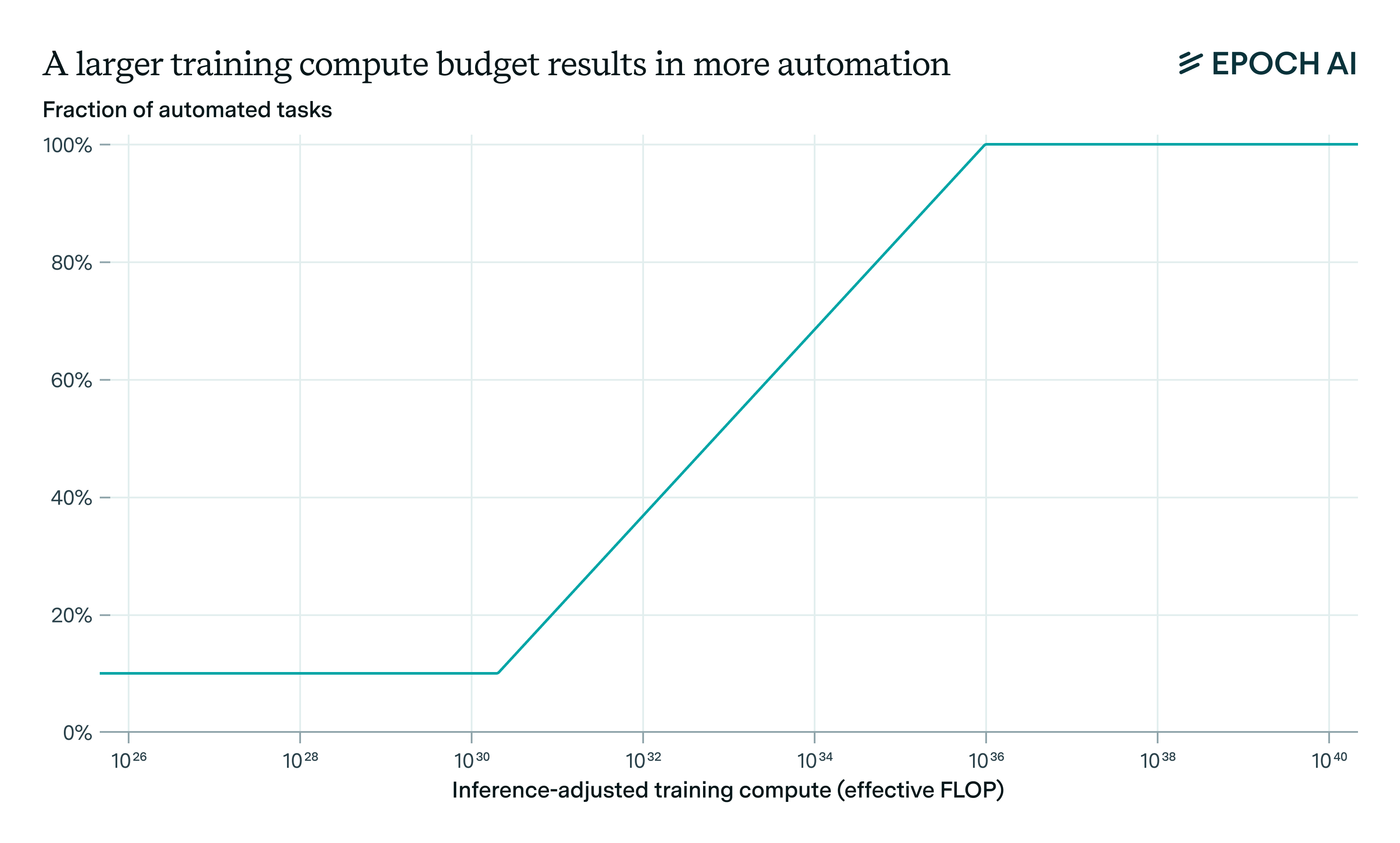
This map implicitly suggests that tasks requiring more effective training compute are fundamentally more “complex” to learn than others. While this includes all economically useful tasks, the GATE model does not specify which tasks are more “complex” than others (and hence which tasks will be automated first).
Runtime assessment
Besides which tasks can be automated, another crucial determinant of the degree of AI automation is how computationally expensive it is to run AI workers. In other words, what are the runtime compute requirements of different automatable tasks?
In the GATE model, this is determined by two main principles. The first is that some tasks fundamentally have greater runtime compute requirements than others. In particular, tasks with a larger task index \(0 \leq i \leq 1\) require more effective inference compute to match the output of a human worker. The minimum task-specific runtime compute requirement is given by a log-linear expression \(10^{\gamma_0 + \gamma_1 i}\). Here \(\gamma_0\) defines the requirements for the easiest to automate task, and \(\gamma_1\) specifies the difference in runtime requirements for the easiest and hardest to automate tasks.
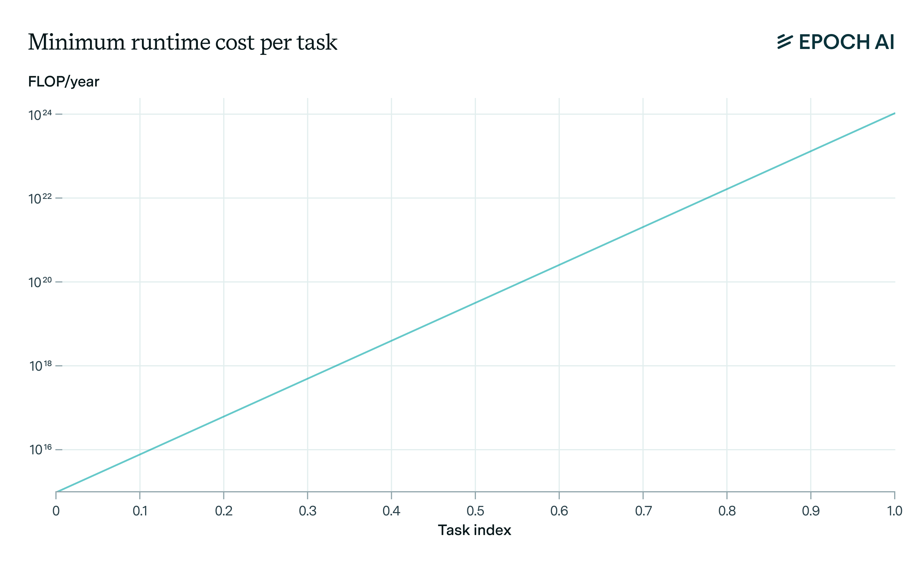
The second core principle is that at each point in time some tasks rely on inference scaling to be automatable, and so have correspondingly higher inference costs. To capture this, we adjust runtime requirements by a task-specific inference multiplier, yielding the following expression for runtime costs:
\[R_i(t) = \underbrace{\max \left(1, \frac{f^{-1}(i)}{C_T(t)} \right)^m}_{\text{Task-specific inference multiplier}} \times \underbrace{10^{\gamma_0 + \gamma_1 i}}_{\text{Minimum runtime cost}}\]Tasks that can only be automated by scaling up inference (i.e. tasks requiring between \(C_T\) and \(C_{T+\iota}\) of effective compute to automate) are subject to an inference cost penalty. This penalty scales with the ratio of the task’s training compute requirements \(f^{-1}(i)\) to the size of the largest training run \(C_T\). As \(C_T\) increases over time, the runtime compute requirements for these tasks decreases until it eventually reaches the minimum runtime cost.
Production
The production module captures the core macroeconomic dynamics of GATE. Crucially, it specifies how automation gets mapped to global economic production, and how investment and allocation decisions are made in the model.
The effective inference compute is allocated across different automated tasks depending on their runtime requirements, determining the number of “digital AI workers” in the economy. AI workers and human workers collectively comprise the total “effective labor” input to economic production. Importantly, labor inputs on non-automated tasks cannot be rapidly scaled up, creating a substantial barrier to rapid expansions in overall production.
Effective labor is then combined with non-AI capital and non-accumulable factors of production (e.g. land or natural resources) to determine the economy’s overall output. Since growing any single input has diminishing returns, production is accelerated when both capital and labor expand in tandem.
Finally, global production (i.e. Gross World Product) is allocated to either consumption, conventional capital investments, or AI investments. The amount of consumption in each timestep is determined to help maximize the utility function of a representative household, via gradient descent.

Labor allocation
The primary mechanism by which GATE allows for a potential dramatic acceleration in economic growth is through a massive increase in the size of the labor force. In particular, in comparison to the human labor force, computation can be scaled up much more quickly, allowing for a huge growth in the number of “AI workers” and economic output.
We quantify the size of the labor force in terms of the “effective labor” \(T\), which is summed across a range of different tasks denoted by the index \(i\). The labor inputs on different tasks \(T_i\) are combined using a standard Constant Elasticity of Substitution (CES) function, where these task inputs are complementary to each other.
\[T(t) = \left( \int_0^1 T_i(t)^{\rho} \, di \right)^{1/\rho} , \, \text{where} \, \rho \in (-\infty, 0).\]In particular, enforcing complementarity between tasks means that we specify that the “substitution parameter” \(\rho\) to be negative. This assumption is key because it captures the famous “Baumol effect”, where limited inputs on one task can bottleneck overall output, and increase the marginal value bottlenecking tasks over time.
As we alluded to in the automation module, some fraction \(f\) of tasks are automated, and can thus be performed by either human workers \(L_i\) or AI workers \(N_i\). In turn AI workers are created via allocating run-time compute to each task, with the creation of an AI worker incurring a task-specific runtime compute cost \(R_i\). The remaining non-automated tasks can only be performed by humans. Formally:
\[T_i(t) = \begin{cases} L_i(t) + N_i(t), & \text{if $i \leq f(t)$}\\ L_i(t), & \text{otherwise} \end{cases}\]There are thus three main pathways to increase the size of the effective labor force: (1) increasing the size of the human labor force, (2) devoting a lot more runtime compute to already automated tasks, and (3) increasing the fraction of automated tasks. As in other models of semi-endogenous growth, we assume that the total amount of human labor \(L\) grows at a constant exponential rate \(g_L\):
\[L(t)=L(0) e^{g_L t}\]In contrast, growth in the effective labor force via pathways (2) and (3) is achieved via automation, which proceeds as described in the previous module.
Add-on: Labor allocation frictions
By default, the GATE model assumes that perfect reallocation of human labor is possible, with workers being able to seamlessly switch from automated to non-automated tasks. One might however object that this assumption is too aggressive, as in reality there are many frictions that increase the time and costs involved in people switching away from automated tasks.
To address this concern, the GATE model includes one alternative extreme scenario: one where zero human labor reallocation is possible. In this case, the labor stock is initially split between different tasks equally, and does not shift at all as task automation proceeds (although we do see constant exponential growth of the human labor force within each task \(i\)):
\[L_i(t) = L_i(0) e^{g_Lt}\]Although neither scenario is realistic, we consider these two extremes as a way to simply evaluate the importance of labor reallocation frictions in the model.
Economic production
With an expanded effective labor force \(T\), the GATE model combines this with conventional capital \(K\) as well as total factor productivity \(A\) to produce economic output \(Y\), i.e. GWP. We also allow GATE to account for potential factors that can’t be scaled up as easily as conventional capital or compute, by including a “non-accumulable” factor of production \(F\) in the production function. This is relatively non-standard, and is added to help illustrate the impact of additional bottlenecks to output growth emanating from long-run non-accumulable factors such as land or natural resources.
The result is a Cobb-Douglas production function with constant returns to scale:
\[Y(t) = T(t)^{1 - \alpha-\mu} K(t)^{\alpha} F(t)^\mu\]Here the constant exponents \(1-\alpha-\mu\), \(\alpha\) and \(\mu\) can be interpreted as output elasticities. The non-accumulable factor becomes important if we set \(\mu>0\), such that we see decreasing returns to scale in effective labor \(T\) and capital \(K\). For simplicity’s sake, the total factor productivity \(A(t)\) is a constant – future versions of GATE will attempt to model productivity growth more realistically.
GWP is then allocated towards three different uses: (1) AI investments (as described in the Compute module), (2) growing the stock of conventional capital, and (3) consumption. As we will see, consumption is especially important because it provides the primary signal for how the GATE model makes its investment and compute allocation decisions throughout the model.
Conventional capital expansion
As in standard macroeconomic models, capital grows endogenously through investment \(I_k\) but is subject to depreciation at a rate \(\delta_K\). As such, the law of motion for capital accumulation is as follows:
\[\dot{K}(t) = I_k(t) - \delta_K K(t)\]Like with compute capital, we also include adjustment costs for conventional capital. This captures the dynamic where trying to rapidly accumulate conventional capital is difficult in the short run. As a result, each dollar of additional investment has a lesser and lesser impact on the capital stock \(K\). However, unlike for compute capital, here we follow the standard of quadratic adjustment costs with an adjustment timescale of \(a_K\), as follows:
\[I_K(t) = I_k(t) + \frac{a_K I_k(t)^2}{2K(t)}\]As usual, higher values of \(a_K\) indicate that costs escalate more rapidly when investment expands quickly. For example, if \(\alpha_K\) is 1 year, investing at a rate of 100% of the current stock per year means that around 70% of the investment is lost to adjustment costs (assuming adjustment costs grow quadratically).
Utility maximization
The final part of the GATE model that brings everything together is the utility function – for simplicity, we adopt the standard assumption that this describes the utility of an average “representative household”. This utility is crucial because it determines all the decisions made by the “social planner” (the key decision-maker in the model), in particular GWP allocations, AI investments, and effective compute allocations.
The social planner chooses consumption, investments and the allocation of compute in order to maximize the utility of the representative household. We follow a standard utility specification from the economics literature, where in each timestep we have isoelastic utility that depends on consumption \(c\), which is then integrated over time to obtain a “lifetime utility”:
\[\max_{\{\mathbf{x}_t\}}\int_{t=0}^{\infty} \exp{\left\{ -(\beta-g_L) t\right\} } \, \, \frac{c(t)^{1-\eta} - 1}{1-\eta} \: dt,\]The parameter \(\eta\) is the relative risk aversion, which captures how much people are willing to shift consumption across time. The overall lifetime utility also depends on the population growth rate \(g_L\), since this influences how many people benefit from consumption in the future, and a time discount rate \(\beta\), which tells us how much people prefer consuming today rather than in the future.
To see how this ties everything together, note that maximizing this objective function means choosing the optimal amount of consumption in each timestep. Optimal consumption depends on economic output, which in turn depends on how much investment there is into AI and conventional capital. It also depends on how AI investment is allocated to increase the effective compute stock, and how this effective compute stock is split between training and inference (impacting the degree of automation). As such, this lifetime utility is central to the entire dynamics of GATE.
In practice, we solve this maximization problem numerically using a gradient-based optimizer, since the model is too complex to be solved analytically.
Beliefs
By default, the GATE model assumes that investors have complete certainty over the future path of automation, including the fact that every task will eventually be automated. However, this may not be the case in practice – among AI researchers and economists, there is frequent disagreement about whether all economically valuable tasks can be automated.
As such, we include an add-on to the GATE model where we can introduce uncertainty over the achievable degree of automation in simulations. In particular, we specify this in terms of the economic decision-maker’s “beliefs” over different scenarios of automation.
Recall that our model has a piecewise log-linear map from compute to the fraction of tasks automated. For the beliefs add-on, we define a certain (user-specified) number of possible such maps, which only differ in terms of the maximum fraction of tasks that can be automated. This is shown below by the different paths, which are identical up until some maximum task automation fraction is reached.
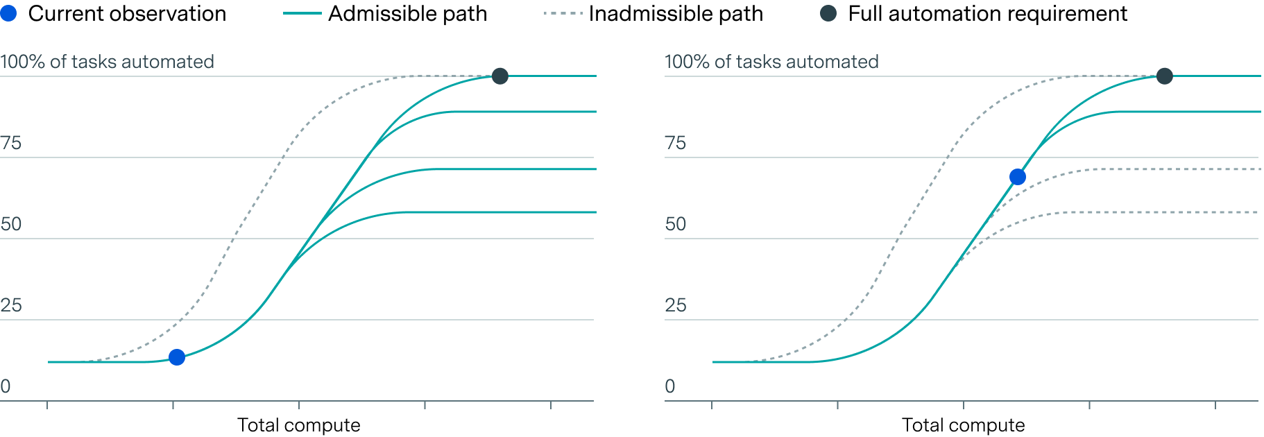
To capture investor beliefs, we therefore specify a discrete number of possibilities for the maximum fraction of automatable tasks, and define a probability mass function over this set of possibilities. To see how this works, consider the following example:
- Initially, investors place a 50% chance on at most 50% of tasks being automatable (i.e. \(f = 0.5\)), 30% chance on \(f = 0.8\) and the remaining 20% on full automation being possible, i.e. \(f=1\).
- Once the fraction of automatable tasks \(f\) exceeds 0.5, the investors “update” their beliefs by splitting the rejected 50% evenly across the remaining two paths, resulting in a 55% chance of at most \(f = 0.8\), and 45% chance of \(f=1\).
- Once \(f\) exceeds 0.8, the investors update once more towards placing 100% probability on full automation being achievable.
In this fashion, this “belief” add-on helps capture potential investor uncertainty over what degrees of automation are possible, which results in less aggressive investment, automation and growth scenarios than the default scenario featuring complete certainty.
Note that regardless of the specified scenario about investor beliefs, our deterministic model assumes that the actual fraction of automatable tasks corresponds to the highest fraction considered in the investor beliefs. So e.g. in the example above 100% automation is always reached. If instead the highest considered fraction was \(f = 0.8\), only 80% of tasks would be automatable in total.
How to interpret the GATE model’s predictions
To interpret the GATE model’s predictions, it’s important to understand how they are meant to be read, and what the model’s limitations are. Notably, the model’s predictions are not meant to represent Epoch AI’s forecasts of future AI developments and economic impacts. As with any economic model, the GATE model’s predictions are instead conditional forecasts, depending on a range of assumptions both in terms of specifications and in terms of parameter values.
In particular, GATE is most useful for analyzing the high-level qualitative dynamics of AI automation, assuming that AI capabilities improvements are solely driven by increases in physical computation and better algorithms. Thus, GATE can be used for deriving stylized facts about the economic impacts of AI automation – in contrast, its quantitative predictions are substantially more uncertain and unreliable.
It is important to note that GATE predictions may be subject to optimization errors. GATE is a complex economic model with a large number of parameters, so the model’s predictions become unreliable for certain parameter ranges due to optimization issues.
Parameters
In this documentation we provide a brief description of each parameter – for more details, please refer to our technical paper.
We split the GATE model’s parameters into three categories:
- AI and compute: Parameters pertaining to the stock of effective compute, as well as to the automation of tasks
- Technological and R&D: Parameters relating to hardware and software R&D
- General economics: Parameters that are commonly used in macroeconomic models
The add-ons to the core model, which account for investor uncertainty, labor reallocation (or lack thereof), and positive externalities in R&D, are described in the model structure section above.
AI and compute parameters
Automation parameters
| Parameter | Symbol | Default | Units |
|---|---|---|---|
| AGI training requirements | \(T\) | 36.5 | eFLOP (OOMs) |
| FLOP gap fraction | \(\Delta f\) | 55 | % |
AGI training requirements
Effective FLOP required to train AI systems capable of automating all tasks.
We take a rough central estimate from (Cotra, 2020), which estimates the computational requirements for training a transformative AI system using “biological anchors” (e.g. from the human brain or evolution), to get 1e36.5 FLOP. This parameter is highly uncertain, so we account for several OOMs of uncertainty ranging from 1e33 to 1e41, based on the distribution of FLOP requirements reported by Cotra.
FLOP gap fraction
This defines the range of effective training compute (adjusted for inference scaling) over which increasing compute increases task automation.
This is defined as a ratio of two quantities - the first quantity is log(AGI training requirements) - log(effective FLOP threshold where more compute leads to more automation). This is divided by the second quantity, given by log(AGI training requirements) - log(initial training compute). This is thus defined as ratio of two quantities measured in OOMs. Formally, this fraction corresponds to
\[\frac{C(100\%) - C(20\%)}{C(100\%) - C(\text{init})},\]where \(C(x\%)\) is the base 10 logarithm of the compute required for \(x\%\) automation. Intuitively, this parameter captures how soon pre-AGI systems start automating the economy. If this parameter is zero, then only AGI can automate anything; if this parameter is one, then we see steady linear progress in automation at current training run sizes.
Since we only have weak evidence for this parameter, we adopt a fairly broad distribution over its values. Some studies suggest that present day AI systems can already automate some tasks that older systems could not (Owen and Besiroglu, 2023), and other sources predict the potential for substantial automatability (Davidson, 2023) or exposure (Eloundou et al., 2023) over the next decade. On current trends, a decade involves 5 OOMs compute scaling (Epoch AI, 2023), i.e. 1e30.5 FLOP. As a FLOP gap fraction for our median training requirements, this results in a FLOP gap fraction of around 0.55.
For the lower end of our range, we note that several AI researchers anticipate rapid improvements in AI capabilities across relatively small scaling of compute. If we assume ~2 OOM of compute could raise AI systems from insignificance to automating half of the economy, then this roughly corresponds to a \(\Delta f \approx 2*2/11~=0.4\) for our range of AGI training requirements \(T\). For our upper end, we consider the situation where 2 more OOMs are needed to reach an increase in the fraction of tasks automated, which results in a fraction of \(\Delta f = (11-2)/11 \approx 0.8\).
Runtime compute parameters
| Parameter | Symbol | Default | Units |
|---|---|---|---|
| Max inference-training compute tradeoff | \(\iota_\text{max}\) | 5 | OOMs |
| Inference-training tradeoff slope | \(m\) | 2 | Dimensionless |
| Minimum runtime compute requirements | \(10^{\gamma_0}\) | 15 | eFLOP/year (OOMs) |
| Task-level runtime compute requirement slope | \(\gamma_1\) | 9 | Dimensionless |
| Initial runtime compute | \(C_I(0)\) | 1e28 | FLOP/year |
Max inference-training compute tradeoff
Maximum value of inference multiplier. This includes effects from both decreasing overtraining and increasing inference scaling, both of which would increase the multiplier (where the “unadjusted runtime compute cost” assumes maximum overtraining).
(Villalobos and Atkinson, 2023) argue that it is possible to increase inference by 2-6 OOMs in exchange for training compute, depending on the type of task. In the opposite direction, it is possible to decrease inference compute by 1 OOM in exchange for more training compute (overtraining). For our central estimate we hence choose 4 + 1 = 5 OOMs.
Inference-training tradeoff slope
Slope of inference compute tradeoff in determining the effective compute size of a system. This captures how many OOMs of inference compute can be substituted for 1 OOM of training compute while achieving the same level of performance.
We base our central estimate of 2 OOMs on the estimates from (Villalobos and Atkinson, 2023), and allow for roughly 2\(\times\) uncertainty, roughly consistent with the provided estimates.
Minimum runtime compute requirements
Minimum runtime compute cost of substituting a worker for the easiest to automate task, at maximum overtraining (i.e. after maximizing training compute to minimize future inference costs).
For this parameter, we anchor loosely to the inference compute required for one of the first automated tasks, namely optical character recognition (OCR). Each forward pass required several hundred thousand to a million mult-adds, and so we loosely anchor to around 1M FLOP per forward pass (e.g. LeNet-4 involved 260k mult-adds per forward pass (Bottou et al., 1994)). Assuming that each forward pass can be used to analyze one character, and around 20 characters are processed per second, this corresponds to around 6e14 FLOP/year, which we round up to 1e15 FLOP/year. There is substantial uncertainty over this parameter (e.g. in terms of which task was automated first, the precise minimum runtime compute requirement, which examples to anchor to, etc.) and so we introduce a range of around 2 OOMs on either side of our central estimate.
Task-level runtime compute requirement slope
Increase in the runtime compute cost in orders of magnitude across tasks, going from automation of the first tasks to full automation.
Compared to the easiest tasks, we assume that the hardest tasks to automate have a computational requirement similar to that of the human brain. To this end, we anchor to (Carlsmith, 2020), who estimates that the human brain does the equivalent of 1e15 FLOP/s, or around 3e22 FLOP/year. Since the brain is known to be highly efficient, we shift this estimate up around 1-2 OOMs to arrive at 1e24 FLOP/year as the minimum runtime compute cost. This parameter is highly uncertain, and as such we account for 2 OOMs of uncertainty on either side of our central estimate.
Initial runtime compute
Total compute available for running AI systems each year, as of the start of 2025.
While the compute devoted to training Gemini Ultra is large by historical standards, the overall compute resources that are not currently dedicated for AI training is substantially larger. For example, (Steinhardt, 2023) estimates the total compute stock to be around 1e29 FLOP,1 and Barnett 2023 similarly estimates that all the AI hardware in the world can produce at most 1e22 FLOP/s (or 3e29 FLOP/year). Both of these values are based on estimates of the quantity of sold microprocessors (e.g. H100 GPUs), and theoretical performance metrics for these processors obtained from official datasheets. However, since in practice it is unlikely that all of this theoretically-available runtime compute can be allocated to AI training, we adjust this estimate down by an OOM to obtain 1e28 FLOP. We account for around 1 OOM of uncertainty above or below this default estimate.
Compute investment parameters
| Parameter | Symbol | Default | Units |
|---|---|---|---|
| Compute adjustment cost exponent | \(\chi\) | 4 | Dimensionless |
| Physical compute limit | \(C_L\) | 2e38 | FLOP/year |
| Compute adjustment timescale | \(\alpha_Q\) | 2 | Years |
| Compute depreciation | \(\delta_Q\) | 30 | %/year |
| Initial largest training run | \(C_T(0)\) | 5e25 | FLOP/year |
| Initial compute investment | \(I_{Q}(0)\) | 2e11 | Dollars |
Compute adjustment cost exponent
Determines how steep the adjustment costs are from increasing the stock of compute. An exponent of 2 means that adjustment costs grow quadratically with investment flows.
The production of AI chips relies on an intricate supply chain that is difficult to expand due to the use of advanced technologies and materials. As a result, supply of compute-related capital is likely highly inelastic, and larger-than-usual premia may need to be paid to expand the compute-related capital stock on a timescale smaller than is typically needed to produce new fabs, datacenters, and lithography machines. Given that we choose quadratic adjustment costs for conventional capital, we assume substantially steeper costs with an exponent from 3 to 5 for compute.
Physical compute limit
Bound on total FLOP that can be performed per year due to thermodynamic limits.
Under the existing CMOS paradigm for microprocessors, computations are generally performed irreversibly, and this results in heat dissipation. As a result, if excessively large quantities of compute are performed in some timeframe, the resulting heat dissipation might be extremely large and have massive environmental effects.
As such, this parameter acts as an upper bound to the FLOP/year. We derive this by combining existing estimates of the maximum FLOP/J of CMOS microprocessors, and estimate a maximum J/year that can be devoted to computation. For the former, (Ho, Erdil and Besiroglu, 2023) estimate that the maximum energy efficiency of CMOS microprocessors is roughly 5e15 FLOP/J. For the latter, we assume that energy availability is capped at 1% of the Earth’s annual energy dissipation, yielding approximately 5e22 J/year based on the Stefan-Boltzmann law.2 If we combine these two results we arrive at a limit of 2e38 FLOP/year.
For the lower end of our range, we consider 2 standard deviations below the ideal CMOS efficiency, and multiply this by the energy consumption of today (i.e. 5e20 J/year (Institute and Smil, 2024)). Thus we have 5e20 J/year * 1.6e14 FLOP/J = 8e34 FLOP/year.
For the higher end of our range, we consider 2 standard deviations above the default ideal CMOS efficiency, and multiply this by 100% of the Earth’s energy budget. This is 5e24 J/year * 1e17 FLOP/year = 5e41 FLOP/year.
Compute adjustment timescale
The adjustment timescale captures how quickly compute investments can be converted into compute stock. For example, if \(\alpha_Q\) is 1 year and we assume that investment costs grow quadratically, investing at a rate of 100% of the current stock per year means that around 70% of the investment is lost to adjustment costs.
This parameter is the counterpart to the capital adjustment timescale \(\alpha_K\), where the reciprocal corresponds to the rate at which the compute stock can be grown before adjustment costs become significant. AI chip manufacturing depends on a complex, hard-to-scale supply chain, featuring sophisticated lithography, advanced packaging, specialized photoresists, and specialized chemicals. Using a sample of 635 fab construction projects between from 1990-2020, (VerWey, 2021) finds that it takes between 1.6 to 2.2 years from fab construction to production depending on the region the fab was constructed in. This suggests that under “normal” conditions when extreme adjustment costs are avoided fab capacity can be substantially expanded just under two years. For the range, we choose values 2\(\times\) larger or smaller than this default estimate.
Compute depreciation
Rate at which compute loses value over time. For example, if \(\delta_Q = 5\%\), then 5% of an existing compute stock is lost each year.
(Ostrouchov et al., 2020) analyzes the reliability and lifetimes of the 18,688 GPUs in the Titan supercomputer at Oak Ridge National Laboratory over its nearly 7 year lifespan from 2012 to 2019. On average, GPUs in the Titan supercomputer lasted around 2.8 years before experiencing failures. However, some units failed much earlier than expected, requiring replacements. GPUs installed in 2017 to replace the failing units lasted significantly longer, often beyond 3 years. The failure rate is \((\text{mean time to failure})^{-1} \approx 0.3\)/year.
Initial largest training run
Largest training run in effective floating point operations (eFLOP) at the start of 2025.
At the time of writing, the largest training run performed was for Google Deepmind’s system Gemini Ultra, at roughly 5e25 FLOP (Epoch AI, 2023). This estimate was obtained by combining two approaches: (1) backing out compute estimates based on known relationships between training compute and performance on certain machine learning benchmarks, and (2) using details of the hardware used during training.3
Initial compute investment
Initial dollar spending on compute production.
Major AI firms spent on the order of $50B per quarter in 2024 (PYMNTS, 2024), so we loosely assume around $200B over the entire year. We account for around 4\(\times\) uncertainty in this parameter.
Technological and R&D parameters
Hardware R&D parameters
| Parameter | Symbol | Default | Units |
|---|---|---|---|
| Hardware R&D returns | \(\lambda_H/\phi_H\) | 5.2 | Dimensionless |
| Returns to scale in hardware R&D | \(\lambda_H\) | 0.14 | Dimensionless |
| Maximum hardware efficiency | \(H^\text{max}\) | 1e23 | FLOP/year/$ |
| Initial hardware efficiency | \(H(0)\) | 1e18 | FLOP/year/$ |
| Initial inputs to hardware R&D | \(I_{H}^{\text{RD}}(0)\) | 1e11 | Real USD/year |
| Initial hardware efficiency growth | \(g_H(0)\) | 27.5 | %/year |
Hardware R&D returns
Measures whether proportional increases in hardware R&D growth result in proportional increases in hardware efficiency growth. Returns remaining greater than 1 results in hyperbolic growth, whereas returns less than 1 yield decelerating progress even with increasing investment.
We follow the estimates in (Davidson, 2023) of the returns, e.g. a median of \(\lambda/\phi = 5.2\) for hardware. This was estimated using GPU data from 2006 to 2022, and dividing the growth rate in FLOP/$ (Cotra, 2020) by the growth rate in cumulative real dollar R&D inputs over the same period (Bloom et al., 2020).
Returns to scale in hardware R&D
Extent to which investments in hardware R&D translate into increases in hardware efficiency. This accounts for two effects, where we think of \(\lambda_H\) as a product of two constants \(\lambda_H = \lambda_H' \cdot \mathcal{p}\). \(\lambda_H' > 1\) corresponds to a network effect where having more R&D inputs yields increasing returns. \(\lambda_H'<1\) is a “stepping on toes” effect where increasing R&D inputs yields diminishing returns. \(\mathcal{p}\) is a constant that accounts for price effects.
For our central estimate of the returns to labor inputs, we anchor weakly to (Erdil et al., 2024). They find a value of around 0.4 for human labor inputs on Stockfish, for which by far the best data was available (here we use the same value of \(\lambda\) as for software R&D). We then multiply this by around 0.35, an elasticity parameter which accounts for price effects, which gives \(0.4 \times 0.35 = 0.14\). For our range, we consider a lower value of \(\lambda_H\) of 0.25 (with elasticity 0.25), and an upper value of 1 (with elasticity 1).
Maximum hardware efficiency
Maximum possible hardware efficiency of AI hardware, based on the current paradigm of CMOS microprocessors.
We estimate this parameter with the same procedure proposed in (Davidson, 2023). In particular, we first determine an upper bound to the FLOP/$ by decomposing it into a product of the energy efficiency in FLOP/J and the inverse of the cost per unit of energy (J/$). The hardware efficiency in FLOP/$/year is then determined by estimating the time range over which hardware is likely to be used, and amortizing the cost of a processor over that time period. For the FLOP/J, (Ho, Erdil and Besiroglu, 2023) proposes a simple model to estimate the limits to the energy efficiency of CMOS processors, which has a geometric mean estimate of around \(5 \times 10^{15}\) FLOP/J at 4-bit precision, with a log-space standard deviation of 0.7 OOMs. Assuming quadratic scaling of energy costs with number precision, this corresponds to around \(3 \times 10^{14}\) FLOP/J at 16-bit precision. If we assume that energy costs can fall from $0.1/kWh today to $0.01/kWh, then we have
\[(5 \times 10^{15} \: \text{FLOP/J}) \cdot (3.6 \times 10^8 \: \text{J/\$}) \approx 10^{24} \: \text{FLOP/\$}\]If we further assume that hardware costs are amortized over 10 years, we arrive at a hardware efficiency of \(10^{23}\) FLOP/year/$. In practice it is unclear whether the optimal substructure assumption that the maximum FLOP/$ can be determined by individually maximizing the FLOP/J and the J/$. It is possible for instance that other bottlenecks may bind prior to reaching limits in FLOP/J or J/$. This introduces uncertainty that goes beyond the uncertainty inherent in the estimates of the FLOP/J, J/$ and amortization period themselves. We allow for a range of 2 OOMs above or below this default estimate, to account for these uncertainties.
Initial hardware efficiency
Computational performance achievable per dollar of hardware spending at the start of 2025.
We anchor our estimate of this parameter to the H100 GPU, which is commonly used for training state of the art AI systems (Lee et al., 2024). It performs around 1e15 FLOP/s (NVIDIA, 2024), and costs around $40k (Leswing, 2023). Over a year, this corresponds to \(1e15 \cdot 365 \cdot 24 \cdot 3600 / 40000 \approx 1e18\) FLOP/year/$. We allow for around 1 order of magnitude of uncertainty in this parameter.
Initial inputs to hardware R&D
Amount spent on improving hardware efficiency per year at the start of 2025.
We obtain a ballpark estimate for this parameter by considering R&D spending from big hardware companies. In 2022, this was $17.5B for Intel (Alsop, 2024), $5.47B for TSMC (Limited, 2022), $5B for AMD (Alsop, 2024), $5.3B for NVIDIA (Macrotrends, 2024), and $3.4B for ASML (Macrotrends, 2024). Since the distribution of hardware R&D spending appears very heavy tailed, we assume a Zipfian distribution with Intel as the leader, and assume there are around 100 firms doing significant hardware R&D worldwide. This results in an estimate of \(\$17.5B \cdot H_{100} \approx \$90B\) for global R&D spending on hardware, where \(H_{100} \approx 5.2\) is the 100th harmonic number. We round this figure up to $100B, and allow for uncertainty around 10x higher or lower than this default estimate.
Initial hardware efficiency growth
The growth rate of hardware efficiency as of the start of 2025.
Our central estimate corresponds to a doubling time of around 2.5 years, which is broadly consistent with the rate of improvement in computational price performance found by (Hobbhahn et al., 2023). We allow for uncertainty ranging from a doubling time of around 2 to 3 years.
Software R&D parameters
| Parameter | Symbol | Default | Units |
|---|---|---|---|
| Software R&D returns | \(\lambda_S/\phi_S\) | 1.25 | Dimensionless |
| Returns to scale in software R&D | \(\lambda_S\) | 0.14 | Dimensionless |
| Maximum software efficiency | \(S^\text{max}\) | 10000 | eFLOP/FLOP |
| Initial inputs to software R&D | \(I_{S}^{\text{RD}}(0)\) | 5e9 | Real USD |
| Initial software efficiency growth | \(g_S(0)\) | 70 | %/year |
Software R&D returns
Measures whether proportional increases in software R&D growth result in proportional increases in software efficiency growth. Returns remaining greater than 1 results in hyperbolic growth, whereas returns less than 1 yield decelerating progress even with increasing investment.
(Erdil et al., 2024) look at a range of domains for software, and find estimates between 0.5 and 3. Additionally (Davidson, 2023) estimates a return to hardware R&D of around 0.8-5, by dividing the growth rate in algorithmic efficiency and the growth in software inputs from (Besiroglu, 2020) - this yields a geometric mean of 2.
Returns to scale in software R&D
The extent which investments in software R&D translate into increases in software efficiency. This accounts for two effects, where we think of \(\lambda_S\) as a product of two constants \(\lambda_S = \lambda_S' \cdot \mathcal{p}\). \(\lambda_S' > 1\) corresponds to a network effect where having more R&D inputs yields increasing returns. \(\lambda_S'<1\) is a “stepping on toes” effect where increasing R&D inputs yields diminishing returns. \(\mathcal{p}\) is a constant that accounts for price effects.
For our central estimate of the returns to labor inputs, we anchor weakly to (Erdil et al., 2024). They find a value of around 0.4 for human labor inputs on Stockfish, for which by far the best data was available (here we use the same value of \(\lambda\) as for software R&D). We then multiply this by around 0.35, an elasticity parameter which accounts for price effects, which gives \(0.4 \times 0.35 = 0.14\). For our range, we consider a lower value of \(\lambda_S\) of 0.25 (with elasticity 0.25), and an upper value of 1 (with elasticity 1).
Maximum software efficiency
Maximum possible software efficiency of AI algorithms.
This parameter is highly speculative, and we are forced to consider several very rough arguments to try and get a handle on its value. (Bubeck and Sellke, 2022) argue that for a Lipschitz-smooth function to fit \(d\)-dimensional data, at least \(n \times d\) parameters are required. For a rough estimate we consider the ImageNet dataset for image classification, which contains \(n \approx 1000\) classes and around \(d \approx 40\) intrinsic dimensions (Pope et al., 2021). We approximate the minimum necessary training compute as \(C \approx 6 ND\), where \(N=n\times d\) is the number of model parameters and \(D\) is the number of datapoints. In this context, we interpret each “datapoint” as a particular “patch” of an image which has been encoded as a vector. Patch dimensions of 8\(\times\)8 pixels are fairly common, and since the most common image size is 500\(\times\)500 (Ehrlich, 2021), this corresponds to around 4000 tokens. If we assume that through algorithmic innovation this can in principle be reduced by an OOM, we are left with 400 tokens. Combining the above results in \(C \approx 6 \cdot (40 \cdot 1000) \cdot (1000 \cdot 400) \approx 1e11\) FLOP. By comparison, the current state of the art system on the ImageNet benchmark, ViT-Huge/14 (Dosovitskiy et al., 2021) was trained with 4e21 FLOP (Epoch, 2024). This thus suggests that ViT-Huge/14, which achieves ~89% top-1 accuracy on ImageNet, could have been trained with around 10 OOM fewer FLOP.
Another approach, followed by (Davidson, 2023) is to consider the situation where roughly 1e36 FLOP is needed to train to AGI (by anchoring to the human brain, based on (Cotra, 2020)), and where this is eventually reduced to the amount of computation done by a human over the first 30 years of life, i.e. 1e24 FLOP. This argument would suggest around 12 OOM of software efficiency gain is possible. It is further possible that algorithms could be improved to be more efficient than the human brain, but we treat this as a rough upper of our range, noting that additional further gains may be possible.
As a third heuristic, (Ho et al., 2024) and (Erdil and Besiroglu, 2022) estimate growth rates of 0.4 OOM/year for algorithmic progress in language models and computer vision respectively. This corresponds to \(\sim\)4 OOM of sustained algorithmic progress since 2014, and it seems broadly reasonable to expect this to persist for another 4 OOMs with greater than 50% probability. From this far removed perspective it is also possible that progress could end up slowing down, but we assign this lower probability. Overall we assume that progress can only be increased further by around 2 OOMs as a loose lower bound.
Overall, there is a tremendous amount of uncertainty over this parameter and as such we consider a wide range of possible values, ranging from 100 to 1e12. For our central estimate, we assume 4 OOMs of progress, but we find a very wide range of values plausible.
Initial inputs to software R&D
Amount spent on improving software efficiency per year, as measured at the start of 2025.
We estimate this based on the number of researchers and researcher salaries, since algorithmic improvements are mainly driven by researcher effort at present. (Benaich and Hogarth, 2019) report around 20,000 unique authors on machine learning papers in 2019, so for a ballpark figure we assume there are 50k researchers in AI today. If each researcher is paid around $100k each, this corresponds to around $5B per year. For lower and upper ranges we consider 5\(\times\) more or less than the default estimate.
Initial software efficiency growth
The growth rate of software efficiency as of the start of 2025.
(Hernandez and Brown, 2020) and (Erdil and Besiroglu, 2022) estimate median doubling times of estimate 16 months and 9 months in image classification algorithms. In language models, (Ho et al., 2024) estimate a median doubling time of 8 months. Algorithmic progress towards AI automating all tasks is likely slower than progress on specific narrow benchmarks, we lean towards longer doubling time estimates, with around a doubling every 16 months. This corresponds to a growth rate of 70%/year. Our uncertainty in this parameter is fairly broad, ranging from a doubling every 8 months to around every 2 years.
General economics parameters
| Parameter | Symbol | Default | Units |
|---|---|---|---|
| Relative risk aversion in isoelastic utility | \(\eta\) | 1.45 | Dimensionless |
| Substitution parameter | \(\rho\) | -0.65 | Dimensionless |
| Output elasticity of capital | \(\alpha\) | 0.35 | Dimensionless |
| Output elasticity of non-accumulable factor | \(\mu\) | 0 | Dimensionless |
| Consumption discount rate | \(\delta\) | 5 | %/year |
| Initial GWP | \(Y(0)\) | 110 | Trillion real USD/year |
| Initial labor force | \(L(0)\) | 3.6 | Billion workers |
| Population growth rate | \(g_L\) | 0.25 | %/year |
| Initial capital stock | \(K(0)\) | 450 | Trillion real USD |
| Adjustment timescale for capital stock | \(\alpha_K\) | 1 | Years |
| Capital depreciation | \(\delta_K\) | 6.5 | %/year |
Relative risk aversion in isoelastic utility
Parameter of the isoelastic utility function \(\frac{c^{1-\eta} - 1}{1-\eta}\) that determines risk preferences. \(\eta=1\) corresponds to taking log utility, and as \(\eta\) increases, consumers become increasingly risk-averse. For example, \(\eta = 2\) suggests indifference between maintaining current consumption, and taking a bet with a 50% chance of doubling consumption and a 50% of decreasing consumption by a third.
A meta-analysis by (Havránek et al., 2015) collects 2,735 estimates of the elasticity of intertemporal substitution (EIS) in consumption. Across 1429 studies for the United States, they find a mean EIS of 0.594 (\(\eta \approx 1.7\)). They find that households in countries with higher income per capita and higher stock market participation show larger values of the EIS. For example, they find an estimated posterior mean of the regression coefficient for income per capita of aorund 0.13, meaning that a doubling of GDP per capita results in an increase in EIS by roughly 0.13. Given the rapid economic growth in our model, we opt for a value of \(\eta\) of 1.5. This also matches with the baseline calibration value of \(2/3\) in the DSGE work of (Smets and Wouters, 2007) (\(\eta = 1.5\)).4
Substitution parameter
Captures how easily labor on different tasks substitute or complement each other. For instance, suppose that \(\rho = -0.5\), and that the labor input is allocated uniformly across different tasks. If the labor input to a third of the tasks is set then to infinity, the total output would increase by 2.25\(\times\). We enforce \(\rho<0\) to ensure that tasks are gross complements.
(Knoblach et al., 2019) measure long-run elasticities of substitutions for the aggregate economy at in the range of 0.45-0.87. We interpolate between the corresponding substitution parameters to obtain \(\frac{1}{2} \left( \frac{0.45 - 1}{0.45} + \frac{0.87 - 1}{0.87} \right) \approx -0.65\). We loosely account for a range of uncertainty, bounded above by -0.2 < 0 so that labor inputs are always gross complements, and bounded below by -5, which suggests very substantial complementarities.
Output elasticity of capital
How much GWP increases for each increase in capital, where \(\text{GWP } \propto \text{ capital}^{\alpha}\). For example, if \(\alpha = 0.5\), a 4\(\times\) increase in capital results in a 2\(\times\) increase in GWP, all else equal.
This is loosely based on (Jones and others, 2003), where estimated capital shares are generally around 0.35, and between 0.2 and 0.6.
Output elasticity of non-accumulable factor
How much GWP would increase for each unit increase in non-accumulable capital, where \(\text{GWP} \propto \text{nature}^{\mu}\). For example, if \(\mu = 0.5\), a 4\(\times\) increase in capital results in a 2\(\times\) increase in GWP, all else equal.
By default, this parameter is chosen to exclude the presence of the non-accumulable factor. To illustrate the significance of the non-accumulable factor, we can also choose \(\mu\) such that the production function has constant returns to scale in all inputs.
Consumption discount rate
The rate at which future consumption is valued less than present consumption. For example, a discount rate of 5% means that the utility from consumption in the next year is worth 95% of the same amount of consumption today.
(Moore et al., 2004) suggest using a social discount rate of 3.5%, and (Zhuang et al., 2007) point out that developed countries tend to use consumption discount rates of 3-7%. We opt for a round number of around 5% as our default parameter estimate, and use 3-7% as our range.
Initial GWP
Gross world product at the start of simulations, i.e., the total economic value produced globally in 2024.
According to the World Bank, the GWP in 2023 was around $106T (The World Bank, 2022). For our defaults we assume around 3% annual GWP growth, resulting in a default of around $110T. For the lower end of the range we use around the 2023 value, and for the upper value we add a buffer of around two more years of 3% growth
Initial labor force
Total number of humans in the labor force at the start of 2025.
According to the World Bank, the labor force in 2023 was 3.6B (The World Bank, 2023). This corresponds to a labor share of around 45%, and we consider lower and upper bounds for the range by considering labor shares of around 42.5% to 47.5% respectively.
Population growth rate
The annual rate of human population increase.
We weight estimated population growth rates by GDP per capita. High-income countries grow \(\sim\)0.1%year, middle income ~1%/year, and low income \(\sim\)3%/year. Since the ratio of high to lower-middle income labor is 3:2, we arrive at around \(\sim\)0.5%/year (United Nations, 2022). We reduce this slightly to 0.25% given the broadly observed trend towards lower birth rates across different countries.
Initial capital stock
Total value of physical capital in the economy at the start of 2025.
We obtain a rough estimate of this based on standard capital depreciation rates and gross savings rates. In particular, global gross savings rates are around 27% of GWP (The World Bank, 2022), and a standard capital depreciation rate is 6% per year (Nadiri and Prucha, 1993). Given that current GWP is \(\sim\) $100 trillion (The World Bank, 2022), we estimate the worldwide capital stock as \(0.27 \cdot \$1e14 \cdot 1/0.06 \approx \$4.5e14\). We assume roughly 2x uncertainty in this number for our overall range.
Adjustment timescale for capital stock
How quickly capital investments can be converted into conventional capital. For example, if \(\alpha_K\) is 1 year, investing at a rate of 100% of the current stock per year means that around 70% of the investment is lost to adjustment costs (assuming adjustment costs grow quadratically).
(Groth, 2005) estimates capital adjustment costs using a similar functional specification on data from the UK economy between 1970-2000, and finds \(\alpha_K\) to be around 1-3. Similarly, (Groth and Khan, 2010) generally report estimates of the adjustment cost parameter to roughly between 0.1 and 10, depending on the data and the precise functional form used. For our purposes we opt for 1 as a rough estimate, and assume a 2\(\times\) factor of uncertainty.
Capital depreciation
The rate at which capital loses value over time. For example, if \(\delta_K = 5\%\), this means 5% of an existing capital stock is lost each year.
The capital depreciation rates are chosen to roughly correspond with the values in (Nadiri and Prucha, 1993) and (Giandrea et al., 2022)
FAQ
What is a FLOP?
A “FLOP” stands for a “FLoating-point OPeration”. This is a unit of computation commonly used when talking about training or running AI systems. Note that this is not the same as FLOP/s (often written as FLOPS), which refers to the number of FLOP per second.
What is effective compute?
“Effective compute” is a measure of the amount of computation available for training or running AI systems, adjusted to account for algorithmic progress. In particular, due to algorithm improvements, it becomes possible to do more with the same amount of computation, which “in effect” has the same impact as increasing the number of computations performed. We measure effective compute in units of effective FLOP (eFLOP), relative to the start of the simulation.
What is effective labor?
The effective labor is the aggregation of the labor contributions of AI and human workers. It roughly corresponds to the amount of human workers that would be needed to produce the same output without AI. It is described in depth in the Production section.
What if some tasks remain unautomated?
By default, we assume that all tasks are automatable given enough effective compute. The beliefs add-on can be used to specify scenarios where full automation is not achievable (e.g. by placing 100% probability on a maximum task automation fraction of 0.8, instead of a max fraction of 1). As long as the fraction of tasks that can be automated is sufficiently large, we still generally observe similar results in the model dynamics up to full automation.
What are the most important parameters of the model?
In our experience with the model, the parameters that matter the most are the AGI training requirements and FLOP gap fraction—which jointly determine the mapping between effective compute and tasks automated—and the hardware and software returns to R&D—which control how costly it is to scale effective compute. In the future we plan to release a sensitivity analysis that further clarifies which parameters influence most the model outcomes.
How did you estimate the default parameters?
Parameters commonly found in economic models (e.g., relative risk aversion) are estimated from the economics literature. AI-related parameters are estimated based on previous work, such as our work on estimating training compute, algorithmic progress, returns to software R&D, etc. The reasoning for the parameter estimates is provided in the Parameters section above and in the accompanying technical paper.
What happens after full automation?
The main focus of GATE is on the dynamics in the leadup towards full automation, and it is likely to make poor predictions about what happens close to and after full automation. For example, in the model the primary value of training compute is in increasing the fraction of automated tasks, so once full automation is reached the compute dedicated to training falls to zero. However, in reality there may be economically valuable tasks that go beyond those that humans are able to perform, and for which training compute may continue to be useful.
Why don’t the model predictions for GWP growth, capital stock, or compute investment match the values of today?
The GATE model uses gradient descent to solve for the optimal allocation of investments and compute, in order to maximize a utility function. The predicted investments near the start of simulations can therefore be quite different from those observed today.
Does GATE take a stance on which tasks will be automated first?
In the model we consider an abstract task space including all economically useful tasks, including both cognitive and physical tasks. However, in GATE we do not take a stance on which tasks are likely to be automated first. Instead, GATE only assumes that there is a fixed spectrum of tasks that require progressively more effective compute at training and inference to be automated. We do not consider bottlenecks inherent to specific tasks, such as physical tasks that require robotics.
Why is the initial fraction of automated tasks nonzero?
We do this so that the initial value of runtime compute is nonzero. Instead, we calibrate the initial fraction based on the current share of GWP that is allocated to runtime compute, which results in approximately 10% of tasks being initially automated.
Acknowledgements
Roles and contributions
Ege Erdil initiated the project, developed the early prototype, and played a central role in advancing the key theoretical and modeling ideas. Andrei Potlogea contributed significantly to the technical exposition and introduced refinements to the economic model. Tamay Besiroglu coordinated the project, contributed to the writing, and ensured alignment across modeling, engineering, and writing efforts. Anson Ho provided ongoing support throughout the project, including calibration of parameter values, general model refinement, and coordinating external feedback. Jaime Sevilla contributed to both the engineering and writing, ensuring coherence between the model’s implementation and its conceptual framework. Matthew Barnett contributed to the writing and parameter settings.
Engineering and sandbox development
Edu Roldán provided technical support on the development of the model. Matej Vrzala contributed to the design of and implemented the interactive sandbox. Andrew Souza supported the implementation of the interactive sandbox. Robert Sandler provided design support, contributing to the usability and presentation of the sandbox interface.
We are grateful to Tyler Cowen, Chad Jones, Ben Golub, Ryan Greenblatt, Kevin Kuruc, Caroline Falkman Olsson, Anton Korinek, Daniel Kokotajlo, Lev McKinney, Daan Jujin, Zachary Brown and Dan Valentine, as well as seminar attendees at the 15th Oxford workshop on Global Priorities Research for their insights and feedback.
-
In particular, (Steinhardt, 2023) estimates that GPT-4 (~1e25 FLOP) was trained on around 0.01% of the world’s compute resources, which suggests an overall runtime compute of around 1e29 FLOP.

-
This says that \(P = \sigma A T^4\), where \(P\) is power, \(\sigma = 5.6 \times 10^{-8} \: \text{Wm}^{-2} \text{K}^{-4}\) is the Stefan-Boltzmann constant, \(A\) is the surface area of the Earth, and \(T\) is the Earth’s surface temperature. (Note that this setup assumes the Earth is an ideal black body with emissivity \(\epsilon = 1\), which does not affect our conclusions.) Assuming the earth has a radius of \(6.4 \times 10^{6}\) m (Mamajek et al., 2015) and surface temperature of 300 K, then we arrive at a rough estimate of \(5 \times 10^{24}\) J/year in annual energy dissipation. Taking 1% of this estimate yields our result.
-
The calculations can be found in this colab notebook.
-
(Elminejad et al., 2022) perform a meta-analysis of papers that estimate the relative risk aversion \(\eta\) using the consumption Euler equation. They find a mean relative risk aversion of around 1 in economics contexts (e.g. \(\eta = 1.2\) under their preferred practice in their table 6), but substantially higher (lower \(\eta\)) in finance contexts.
About the authors









Related work

